Home Blog Page 2

Introducing Groq One of The Fastest LLM Chats

In the rapidly advancing realm of artificial intelligence, speed and efficiency are not just goals; they are imperatives. As AI models grow increasingly complex, the quest for faster, more responsive computing has led to a groundbreaking innovation: Groq’s Tensor Streaming Processor (TSP), a Linear Processor Unit (LPU) that stands poised to redefine the landscape of AI computations. With response times clocking in at an astonishing rate of nearly 500 T/s, Also note that Grok is NOT an LLM, the underlying models are Mixtral or Llama the improvment is performance in due to hardware not algorithmically.

Traditional GPUs, with their parallel processing capabilities and multitude of cores, have long been the standard bearers in the field of AI and graphics rendering. However, these GPUs operate on the SIMD (Single Instruction, Multiple Data) model, a structure that, while powerful, comes with its own set of complexities, particularly when it comes to scheduling and latency. Enter Groq’s LPU, a novel design that sidesteps these issues by adopting a deterministic performance model specifically catered to AI workflows.

The LPU’s architecture eschews the conventional approach in favor of a streamlined, every-clock-cycle-counts design, ensuring a level of consistent latency and throughput that was once thought unachievable. For developers, this translates to unprecedented precision in performance prediction and optimization, a pivotal advantage for real-time AI applications.

This design is not only a beacon of performance but also of energy efficiency. By eliminating the need to manage multiple threads and by maximizing core utilization, the LPU ensures more computations per watt than ever before. Energy efficiency, combined with the LPU’s scalability—wherein multiple TSPs can be seamlessly linked without the common bottlenecks present in GPU clusters—heralds a new era of simplified hardware expansion for large-scale AI models.

The implications extend far beyond mere technical specs. LPUs promise to shape the future of AI application serving, offering a robust alternative to the highly sought-after A100s and H100s. With Groq’s TSP, we stand on the precipice of a transformative leap in performance—one that could very well accelerate the pace of AI innovation and broaden the horizons of what is computationally possible.

Potential Applications

Autonomous agents

Building autonomous agents, for example something with LangChain stands to gain substantially from the increased token per second (T/s) processing capabilities provided by advanced processors like Groq’s Tensor Streaming Processor (TSP). Autonomous agents, ranging from virtual assistants to sophisticated robots, require rapid processing of data to interact with their environment effectively and make autonomous decisions. Here’s how faster T/s can be beneficial in this context:

  1. Real-Time Decision Making: Autonomous agents must process a vast array of inputs to make decisions in real time. The faster T/s rate allows for quicker analysis of sensor data, which is critical for agents that operate in dynamic or unpredictable environments.
  2. Improved Perception: Agents rely on processing visual, auditory, and other sensory data to perceive their surroundings. Accelerated T/s rates can lead to more advanced perception capabilities, enabling agents to understand and react to complex scenarios with higher accuracy.
  3. Interactive Learning: Machine learning algorithms, especially those involving reinforcement learning where an agent improves through trial and error, can greatly benefit from faster processing. With more computations per second, agents can iterate and learn from interactions much quicker.
  4. Advanced Natural Language Understanding: For agents that interact with humans, rapid T/s enables sophisticated language models to parse, understand, and generate language in real-time, leading to more natural and fluid conversations.
  5. Dynamic Path Planning: In robotics, quick processing speeds can facilitate more efficient path planning and obstacle avoidance, as the agent can reassess and adjust its trajectory instantaneously in response to changes in the environment.
  6. Enhanced Multi-agent Coordination: Faster T/s processing can improve the coordination among multiple autonomous agents, such as a fleet of drones or autonomous vehicles, allowing them to operate in harmony and respond to each other’s actions promptly.
  7. Human-like Reflexes: When speed is critical, such as in medical robots or in disaster response scenarios, the ability for an autonomous agent to respond quickly and appropriately can make the difference in outcomes.
  8. Robust Simulations for Training: Training autonomous agents often involves simulations that can be computationally intensive. High T/s rates can make these simulations more efficient, leading to better-trained agents in a shorter amount of time.

The development of autonomous agents that can respond and adapt to their environment in real time is a challenging task, and the demand for computational speed is ever-present. With the advancements in processors and higher T/s rates, it is becoming increasingly possible to create agents that are not only responsive and efficient but also capable of complex, nuanced interactions and behaviors that more closely mimic human-like intelligence.

How Did Groq Do It?

Groq’s LPU (Linear Processing Unit) is faster and more energy-efficient than Nvidia GPUs for inference tasks. Unlike Nvidia GPUs, which require high-speed data delivery and High Bandwidth Memory (HBM), Groq’s LPUs use SRAM, which is 20 times faster and consumes less power. Groq’s LPUs also use a Temporal Instruction Set Computer architecture, reducing the need to reload data from memory and avoiding HBM shortages. Groq claims that its technology could replace GPUs in AI tasks with its powerful chip and software, potentially eliminating the need for specialized storage solutions. Does this mean LLM’s were the killer app for TPU clouds?

This tweet goes more in-depth of their hardware.

OpenAI Releases Sora Text-to-Video

Unless your living under a rock, in the world of AI OpenAI has released their first text-to-video model and it is impressive.

Sora is an AI model developed by OpenAI that can create realistic and imaginative scenes from text instructions. It is a text-to-video model capable of generating videos up to a minute long while maintaining visual quality and adherence to the user’s prompt. Sora is designed to understand and simulate the physical world in motion, with the goal of training models that help people solve problems requiring real-world interaction. The model can generate complex scenes with multiple characters, specific types of motion, and accurate details of the subject and background.

Examples

Sora can generate multiple videos side-by-side at the same time.

Sora can combine videos

Sora can follow up and edit videos.

The Architecture

According to Sora’s technical report, Sora’s architecture involves turning visual data into patches, compressing videos into a lower-dimensional latent space, training a network that reduces the dimensionality of visual data, and extracting a sequence of spacetime patches which act as transformer tokens. Sora is a diffusion model that scales effectively as a video model and can generate videos with variable durations, resolutions, and aspect ratios. It can also be prompted with other inputs, such as pre-existing images or video, enabling a wide range of image and video editing tasks. Additionally, Sora exhibits emerging simulation capabilities, such as 3D consistency, long-range coherence, object permanence, interacting with the world, and simulating digital worlds. However, it also has limitations in accurately modeling the physics of basic interactions and other failure modes.

Sora is a comprehensive diffusion transformer model that processes text or images and generates video pixel output. By analyzing vast volumes of video data using gradient descent, Sora acquires an internal understanding of physical dynamics, essentially forming a trainable simulation or “world model.” While Sora doesn’t directly integrate Unreal Engine 5 (UE5) into its processing loop, it can incorporate text and video pairs created with UE5 into its training data as synthetic examples.

Limitations

Sora’s emergent physics understanding is still fragile and imperfect.

Despite extensive research and testing, OpenAI acknowledges that it cannot predict all the beneficial ways people will use the technology, nor all the ways people will abuse it. The model is based on a diffusion architecture and uses a transformer architecture similar to GPT models. It builds on past research in DALL·E and GPT models, using the recaptioning technique from DALL·E 3 to follow the user’s text instructions in the generated video more faithfully. Sora serves as a foundation for models that can understand and simulate the real world, a capability believed to be an important milestone for achieving AGI.

Putting Together an OpenAI Agent With LlamaIndex 

Thanks to the new OpenAI API that supports function calling, creating your own agent has never been easier!

In this tutorial notebook, we’ll demonstrate how to build an OpenAI agent in just 50 lines of code or less. Despite its brevity, our agent is fully-featured and capable of carrying on conversations while utilizing various tools. Using LlamaIndex we will bu agent that will get the current price of a stock using the Yahoo Finance API.

Setting Up

The main thing we need is:

  1. the OpenAI API (using our own llama_index LLM class)
  2. a place to keep conversation history
  3. a definition for tools that our agent can use.

If you’re opening this Notebook on colab, you will probably need to install LlamaIndex 🦙.

%pip install llama-index-agent-openai
%pip install llama-index-llms-openai
!pip install llama-index

Next, we need to set up the foundation for working with LlamaIndex agents, tools, and OpenAI’s LLMs, while also ensuring proper asynchronous execution.

import json
from typing import Sequence, List

from llama_index.llms.openai import OpenAI
from llama_index.core.llms import ChatMessage
from llama_index.core.tools import BaseTool, FunctionTool

import nest_asyncio

nest_asyncio.apply()

Here we will create a function using the Yahoo Finance API, to get the current price of a stock.

import yfinance as yf
from functools import cache

@cache
def get_stock_price(ticker: str) -> Union[float, None]:
  """
  Retrieves the current price of a stock using yfinance, with caching for performance.

  Args:
    ticker: The ticker symbol of the stock.

  Returns:
    The current price of the stock, or None if an error occurs.
  """
  try:
    stock = yf.Ticker(ticker)
    return stock.info["regularMarketPrice"]
  except (yf.YFException, KeyError) as e:
    print(f"Error retrieving price for {ticker}: {e}")
    return None

stock_tool = FunctionTool.from_defaults(fn=stock)

Agent Definition

Now, we define our agent that’s capable of holding a conversation and calling tools in under 50 lines of code.

The meat of the agent logic is in the chat method. At a high-level, there are 3 steps:

  1. Call OpenAI to decide which tool (if any) to call and with what arguments.
  2. Call the tool with the arguments to obtain an output
  3. Call OpenAI to synthesize a response from the conversation context and the tool output.

The reset method simply resets the conversation context, so we can start another conversation.

class YourOpenAIAgent:
    def __init__(
        self,
        tools: Sequence[BaseTool] = [],
        llm: OpenAI = OpenAI(temperature=0, model="gpt-3.5-turbo-0613"),
        chat_history: List[ChatMessage] = [],
    ) -> None:
        self._llm = llm
        self._tools = {tool.metadata.name: tool for tool in tools}
        self._chat_history = chat_history

    def reset(self) -> None:
        self._chat_history = []

    def chat(self, message: str) -> str:
        chat_history = self._chat_history
        chat_history.append(ChatMessage(role="user", content=message))
        tools = [
            tool.metadata.to_openai_tool() for _, tool in self._tools.items()
        ]

        ai_message = self._llm.chat(chat_history, tools=tools).message
        additional_kwargs = ai_message.additional_kwargs
        chat_history.append(ai_message)

        tool_calls = ai_message.additional_kwargs.get("tool_calls", None)
        # parallel function calling is now supported
        if tool_calls is not None:
            for tool_call in tool_calls:
                function_message = self._call_function(tool_call)
                chat_history.append(function_message)
                ai_message = self._llm.chat(chat_history).message
                chat_history.append(ai_message)

        return ai_message.content

    def _call_function(self, tool_call: dict) -> ChatMessage:
        id_ = tool_call["id"]
        function_call = tool_call["function"]
        tool = self._tools[function_call["name"]]
        output = tool(**json.loads(function_call["arguments"]))
        return ChatMessage(
            name=function_call["name"],
            content=str(output),
            role="tool",
            additional_kwargs={
                "tool_call_id": id_,
                "name": function_call["name"],
            },
        )

The agent serves as a bridge between the user and the LLM, managing conversation flow and tool integration. Tools extend the agent’s capabilities with custom functions. The agent maintains a chat history for context. It handles tool calls requested by the LLM, enabling dynamic interactions.

agent = YourOpenAIAgent(tools=[stock_tool])
agent.chat("Hi")
'Hello! How can I assist you today?'
agent.chat("What is the stock price of appl")

LlamaIndex has different implementation methods, some better than others. For example, they provide an OpenAIAgent .

OpenAIAgent 

This agent implementation not only adheres to the BaseChatEngine and BaseQueryEngine interfaces, making it seamlessly compatible with the LlamaIndex framework, but also boasts several advanced features such as support for multiple function calls per conversation turn, streaming capabilities, async endpoints, and callback and tracing functionality.

from llama_index.agent.openai import OpenAIAgent
from llama_index.llms.openai import OpenAI
llm = OpenAI(model="gpt-3.5-turbo-0613")
agent = OpenAIAgent.from_tools(
    [multiply_tool, add_tool], llm=llm, verbose=True
)

Streaming Chat

One key advantage is the ability to receive responses in a streaming fashion, allowing for incremental and real-time interaction with the model. This can be particularly useful for applications where immediate feedback or step-by-step processing is required, such as in conversational interfaces, real-time translation, or content generation. Additionally, streaming chat supports async endpoints, callback and tracing, and async streaming chat, providing flexibility and efficiency in handling conversations and responses

response = agent.stream_chat(
    "What is 121 * 2? Once you have the answer, use that number to write a"
    " story about a group of mice."
)

response_gen = response.response_gen

for token in response_gen:
    print(token, end="")

Google Releases Gemini 1.5 With 10M Context Window

Google has released its next-generation AI model, Gemini 1.5. It is a significant advancement over the previous model, Gemini 1.0 Ultra, and offers dramatic improvements across various dimensions. Gemini 1.5 Pro, the first model released for early testing, achieves comparable quality to 1.0 Ultra while using less compute. This is just 2 months after the initial release of Gemini.

One of the key breakthroughs is its long-context understanding, with a capacity to process up to 1 million tokens, enabling entirely new capabilities and applications for developers and enterprise customers. The model is built upon leading research on Transformer and Mixture-of-Experts (MoE) architecture, making it more efficient to train and serve. It also delivers enhanced performance, outperforming its predecessor on 87% of the benchmarks used for developing large language models (LLMs). Additionally, extensive ethics and safety testing have been conducted to ensure responsible deployment of the model.

Gemini 1.5 is Here

This is one of the most shocking examples:

With only instructional materials (500 pages of linguistic documentation, a dictionary, and ≈ 400 parallel sentences) all provided in context, Gemini 1.5 Pro is capable of learning to translate from English to Kalamang, a language spoken by fewer than 200 speakers in western New Guinea in the east of Indonesian Papua2 , and therefore almost no online presence. Moreover, we find that the quality of its translations is comparable to that of a person who has learned from the same materials.

– Gemini 1.5 is Google’s next-generation AI model, offering significant improvements over the previous model, Gemini 1.0 Ultra.

– It achieves comparable quality to 1.0 Ultra while using less compute and introduces a breakthrough in long-context understanding, with a capacity to process up to 1 million tokens.

Architecture

Gemini 1.5 is a state-of-the-art deep learning model built on top of cutting-edge research in Transformer and MoE (Model Parallelism with Experts) architectures. Unlike traditional Transformers that use one large neural network, MoE models are composed of smaller “expert” networks.

MoE models dynamically activate only the most relevant expert pathways within their neural network based on the input they receive, significantly improving efficiency compared to conventional approaches. Google has been at the forefront of developing and implementing MoE techniques for deep learning through various groundbreaking research papers like Sparsely-Gated MoE, GShard-Transformer, Switch-Transformer, M4, and more.

Gemini 1.5 leverages these advancements in model architecture to learn complex tasks faster while maintaining high-quality results. It is also more efficient during both training and serving phases. These efficiencies enable our teams to iterate quickly, train advanced versions of Gemini rapidly, and continue working towards further optimizations.

Impressive Context lengths

The Impressive Context lengths of Gemini 1.5 cannot be overstated, especially when it pertains to navigating the complex and dense world of codebases. With the ability to process up to 1 million tokens, which is over 30K lines of code, it now means the model has dramatically expanded the horizon of possibilities for software development and maintenance. Programmers and engineers can now leverage this AI to understand and work with larger sections of code in a single instance, allowing for a more comprehensive analysis and quicker troubleshooting. Not only that but equally if not more impressive is its near-perfect retrieval accuracy. This ensures that the most relevant and useful information is available when needed, minimizing the risk of overlooking crucial details inherent in massive code repositories and hallucinations.

This technological leap places significant competitive pressure on Retrieval-Augmented Generation (RAG) models, which may struggle to keep up with the vast context window and precision of Gemini 1.5. Google’s tech report suggests that performance remains robust even when scaling up to staggering sizes like 10 million tokens. As developers embrace this expansion in context size, they’re unlocking opportunities for AI-assisted programming that were once considered science fiction. However, the cost of managing such a voluminous stream of tokens remains a topic for discussion. The financial and computational resources required to sustain these capabilities are substantial, and whether they justify the benefits is yet to be seen. Additionally, the future of Gemini hints at an evolution toward multi-modal learning, with plans to ingest various media types such as files and videos, further enriching the context and utility of the AI — a step beyond its current limitation to image inputs.

StabilityAI Releases Stable Cascade

StabilityAI has made a new contribution with the introduction of Stable Cascade—a cutting-edge text-to-image model that is set to redefine the way we interact with AI-generated visuals. Tailored for enthusiasts and developers alike, Stable Cascade stands out by being released under a non-commercial license, which opens the doors for countless non-commercial applications and learning opportunities.

Image made by X user @cocktailpeanut with Stability Cascade

This model leverages a three-stage approach, making it not only groundbreaking but also exceptionally user-friendly in terms of training and fine-tuning—even on standard consumer hardware. The creators of Stable Cascade have revolutionized the field with their hierarchical compression technique, which facilitates the creation of high-quality images from a highly compressed latent space. This offers a powerful and efficient method for generating images that could potentially transform the industry.

Not just that but, Stable Cascade has been engineered to provide seamless integration with the diffusers library, ensuring that users can employ the model for inference with ease. In a move to foster transparency and collaboration, StabilityAI has made the model’s training and inference code publicly accessible on their GitHub page.

Features of Stable Cascade

What sets Stable Cascade apart is its unique architecture, which consists of three distinct stages—A, B, and C—that work in concert to produce exceptional outputs. This departure from the Stable Diffusion models showcases StabilityAI’s commitment to innovation and versatility within the AI space.

Adding to its impressive capabilities, the model offers additional features such as image variations and image-to-image generation. These features not only enhance the creative possibilities but also demonstrate the flexibility of the model to cater to a wide range of artistic and practical applications.

The comprehensive release of Stable Cascade does not stop at the model itself. It includes all the necessary code for training and fine-tuning, accompanied by tools like ControlNet and LoRA, which aim to lower the barriers to further experimentation and refinement of this already remarkable architecture.

As StabilityAI unveils Stable Cascade to the world, the potential for creativity and innovation in the realm of text-to-image models takes a monumental leap forward, promising to unlock new possibilities for creators and developers alike.

Stable Cascade’s Unique Architecture

Stable Cascade is a new text to image model released by Stability AI. It is built on a three-stage architecture, comprising Stages A, B, and C, which allows for a hierarchical compression of images, achieving remarkable outputs while utilizing a highly compressed latent space. The model is exceptionally easy to train and finetune on consumer hardware, and it is being released under a non-commercial license that permits non-commercial use only.

The three stages of the Stable Cascade architecture are:

  • Stage A: This stage generates a low-resolution version of the image.
  • Stage B: This stage refines the image from Stage A and adds more detail.
  • Stage C: This stage generates the final, high-resolution image.

Stable Cascade introduces an interesting three-stage approach, setting new benchmarks for quality, flexibility, fine-tuning, and efficiency with a focus on further eliminating hardware barriers. The model is available for inference in the diffusers library. The architecture of Stable Cascade allows for additional training or finetuning, including ControlNets and LoRAs, to be completed singularly on Stage C, which comes with a 16x cost reduction compared to training a similar-sized Stable Diffusion model. The model’s modular approach helps keep the expected VRAM requirements for inference to approximately 20gb but can be further lowered by using the smaller variants. Stable Cascade performs best in both prompt alignment and aesthetic quality in almost all model comparisons.

In addition to standard text-to-image generation, Stable Cascade can generate image variations and image-to-image generations. The release includes all the code for training, finetuning, ControlNet, and LoRA to lower the requirements to experiment with this architecture further.

Final Thoughts

The model overall looks promising. It seems to do pretty well with text in images, something AI has seemed to strugle with. However, most AI image models are getting better at it. Ideogram was one of the first to release decent text in images, then came DALL-E 3 and eventually Midjourney.

My concern with these models has always been whether they can be freely downloaded and fucked around with. As long as the community is able to get their hands on them and fine-tune them, train new base models and LoRAs, and just generally break them in new and unexpected ways, then the existence of a commercial license seems completely fine to me. From what I’ve seen it works better. not 100% perfect, but hands and text seem a lot better finally.

While I’m excited about the new base model and architecture from Stability AI, which is akin to SD 1.5, SDXL, and Cascade in terms of being a foundational model that needs fine-tuning by the open-source community, there’s one concern weighing on my mind. Specifically, it’s the $20/month licensing fee – if I have to pay this even without generating any net earnings from a project, it could make devs pause before diving in. Ideally, I’d prefer a structure where I only need to pay once my earnings can cover the cost. It’s worth noting that Stability AI is currently losing $8 million per month and relies heavily on support from its community for survival. Nonetheless, stability remains crucial as it ensures continued progress in this field.

Nvidia Releases Chat with RTX

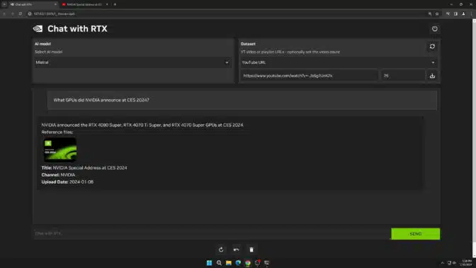
Nvidia just released Chat with RTX, an open sourced local AI Chatbot for PCs Powered by Its Own GPUs: This is from Nvidia’s new technology demo called “Chat with RTX” that allows users to use open-source AI large-language models to interact with their local files and documents.

An AI chatbot that runs locally on your PC

Nvidia has released chat with RTX, in a tech demo they showed what allows users to personalize a chatbot with their own content, accelerated by a local NVIDIA GeForce RTX 30 Series GPU or higher with at least 8GB of video random access memory, or VRAM. The tool uses retrieval-augmented generation (RAG), NVIDIA TensorRT-LLM software, and NVIDIA RTX acceleration to bring generative AI capabilities to local, GeForce-powered Windows PCs.

Users can connect local files on a PC as a dataset to an open-source large language model, enabling queries for quick, contextually relevant answers. The tool supports various file formats and allows users to include information from YouTube videos and playlists. Chat with RTX runs locally on Windows RTX PCs and workstations, providing fast results, and ensuring that the user’s data stays on the device. It requires a GeForce RTX 30 Series GPU or higher with a minimum 8GB of VRAM, Windows 10 or 11, and the latest NVIDIA GPU drivers. The app is built from the TensorRT-LLM RAG developer reference project, available on GitHub, and developers can use the reference project to develop and deploy their own RAG-based applications for RTX, accelerated by TensorRT-LLM.

Open Source Continues

The release of Chat with RTX is a testament to the ongoing commitment Nvidia has to the open-source community. The decision to allow local processing of AI applications opens up a new frontier for developers and enthusiasts alike. By running these models locally, users have greater control over their privacy and data security while still tapping into the power of cutting-edge AI.

With the compatibility of open-source models like Mistral and Llama, users can now leverage the power of Nvidia GPUs to run sophisticated large-language models directly on their PCs. This local approach is not only a boon for privacy but also for performance, as it reduces the latency typically associated with cloud-based services. As users interact with these AI models, their feedback and modifications can contribute to the larger pool of knowledge, fostering a collaborative environment for improvement and growth.

Closing Thoughts

Nvidia’s latest move with Chat with RTX is nothing short of a bold stride into a future where local AI processing becomes as commonplace as the graphics processing we’ve become accustomed to. The thought of models meticulously optimized for maximum performance on specific hardware is an attractive one. There’s something deeply satisfying about the economy of resources—no excess, no waste—just pure, streamlined efficiency. Nvidia’s understanding of this is clear; by refining their GPUs to tailor-fit the demands of large language models (LLMs), they’re maximizing the value that users get out of their hardware.

This optimization goes beyond sheer performance. It’s the realization that they don’t need to license their GPU architectures to third parties to make an impact in the AI space. Instead, they can be the direct LLM provider, leveraging their hardware expertise to craft a user-friendly AI ecosystem. The integration of desktop retrieval-augmented generation (RAG) is particularly exciting. Historically, local UIs have either overlooked this feature or tacked it on as an afterthought. Nvidia’s holistic approach indicates a keen understanding of what users want and need.

From a personal standpoint, I am thrilled by the user-friendly aspect of their new technology. The ability to easily upload and train one’s own datasets is often considered an advanced task, yet Nvidia appears to making this beginner friendly. For beginners looking to dip their toes into the world of customized AI, this approachability is a significant draw.

Nonetheless, it’s important to recognize that the concept of running a local model, even one powered by RAG, is not necessarily for those with the right hardware. However, Nvidia distinguishes itself not through the novelty of the idea, but in the execution—delivering a seamless, accessible experience for a broad audience.

Reka Releases Reka Flash, a Highly Capable Multimodal Model

In the ever-evolving landscape of AI, Reka is setting a new standard with the unveiling of Reka Flash, an exceptional multimodal and multilingual model designed for efficiency and speed. Emerging as a “turbo-class” contender, the 21-billion parameter powerhouse, Reka Flash, has been meticulously trained from the ground up to push the boundaries of AI capabilities. It stands out in the marketplace with its ability to rival the performance of much larger contemporaries, striking a formidable balance between agility and quality. This makes it an ideal solution for demanding applications that necessitate rapid processing without compromising on output excellence.

As Reka solidifies its position in the high-performance AI arena, Reka Edge offers a compact alternative. With a 7-billion parameter construct, it’s tailored for environments where efficiency is paramount. Whether deployed on devices or utilized locally, Reka Edge promises to deliver robust AI capabilities without the heft of its larger counterparts.

Available for exploration in the Reka Playground through a public beta, Reka Flash and Reka Edge are poised to redefine what’s possible in the intersection of language comprehension and visual perception. And for those looking to push the envelope even further, Reka teases the arrival of its most ambitious project yet, Reka Core, set to launch in the coming weeks.

Overview of Reka’s new AI model

As per their benchmarks, he models include Reka Flash, Gemini Pro, GPT-3.5, Grok-1, Mixtral 45B, Llama-2, GPT-4, and Gemini Ultra. The benchmarks include MMLU, GSM8K, HumanEval, and GPQA.

Here are some of the key things you can tell from the benchmark:

  • Reka Flash performs well on all four benchmarks, but it is not the best model on any of them.
  • Reka Flash is a relatively small model (21B parameters), but it is able to achieve competitive performance with much larger models.
  • The best model on a particular benchmark depends on the specific task that the model is being used for.

Overall, their results shows that their model is pretty powerful for its size.

Reka Multimodal Capabilities

Reka Flash performs well across the board on the listed benchmarks. It’s also worth noting that this table only shows a small sample of benchmarks. There are many other factors to consider when evaluating a language model, such as its training data, its architecture, and its computational efficiency.

Testing The Model

First let’s start off by giving it a simple coding question.

Ok not bad. Not let’s ask it a hard question.

This question was pulled from Leetcode 2751 Robot Collisions. Notice how I didn’t mention Leetcode or the question tile in the prompt? I did this so we can try and make sure there the question wasn’t seen in its training data by chance. I also tried to pick a relatively newer question, so the chances of it being in its data were even less. Nonethless, here is the result we got. It seemed to have gotten the correct parameters, it just has a different name function and no return types. hWich makes sense, considering we just asked the raw question.

I will post the rest of the answer here in case you want to copy it:

def survivingRobots(positions, healths, directions):
    i = 0
    while i < len(positions) - 1:
        j = i + 1
        while j < len(positions):
            if directions[i] == 'L' and positions[i] == positions[j]:
                if healths[i] < healths[j]:
                    healths[i] -= 1
                elif healths[i] > healths[j]:
                    healths[j] = 0
                else:
                    healths[i] = 0
                    healths[j] = 0
                j += 1
            elif directions[i] == 'R' and positions[i] == positions[j]:
                if healths[i] < healths[j]:
                    healths[j] -= 1
                elif healths[i] > healths[j]:
                    healths[i] = 0
                else:
                    healths[i] = 0
                    healths[j] = 0
                j += 1
            else:
                i += 1
                j += 1
    return [h for h in healths if h > 0]

Unfortunately when it was ran it only passed 128 / 2433 testcases. Albeit it’s a hard question and most language models probably wouldn’t get it first shot.

Testing Reka Flash’s v1.0

The result:

<table>
 <thead>
  <tr>
   <th>IdNum</th>
   <th>LName</th>
   <th>FName</th>
   <th>JobCode</th>
   <th>Salary</th>
  </tr>
 </thead>
 <tbody>
  <tr>
   <td>1876</td>
   <td>CHIN</td>
   <td>JACK</td>
   <td>TA1</td>
   <td>$44,096</td>
  </tr>
  <tr>
   <td>1114</td>
   <td>GREENWALD</td>
   <td>JANICE</td>
   <td>ME3</td>
   <td>$38,950</td>
  </tr>
  <tr>
   <td>1556</td>
   <td>PENNINGTON</td>
   <td>MICHAEL</td>
   <td>ME1</td>
   <td>$31,054</td>
  </tr>
  <tr>
   <td>1354</td>
   <td>PARKER</td>
   <td>MARY</td>
   <td>FA3</td>
   <td>$67,445</td>
  </tr>
  <tr>
   <td>1130</td>
   <td>WOOD</td>
   <td>DEBORAH</td>
   <td>PT2</td>
   <td>$37,427</td>
  </tr>
 </tbody>
</table>

This was very impressive. Seems to have very good OCR under the hood. Go ahead and test the code yourself and compare it to the table.

Closing Thoughts

The arrival of Reka Flash is indeed a noteworthy leap in the realm of artificial intelligence, presenting itself as a fairly impressive model with considerable potential. As a testament to its capabilities, my initial interaction with the model suggests there’s much to be explored and harnessed within its sophisticated architecture. However, to fully grasp the extent of its prowess, further experimentation and exploration are essential.

While Reka Flash positions itself as a high-caliber model, it’s important to note that this isn’t the pinnacle of Reka’s innovation. The impending release of Reka Core looms on the horizon, teasing the promise of an even more powerful tool in the AI toolkit. Given what we’ve seen from Reka Flash and Reka Edge, expectations are high for what Reka Core will bring to the table.

The anticipation of Reka Core brings about contemplation of Reka’s trajectory among the constellation of companies in the LLM (large language model) space. It’s an arena filled with heavyweights and emerging challengers, each vying to push the boundaries of what’s possible. In such a competitive market, Reka’s strategy and offerings will be crucial factors.

An unfortunate caveat to the excitement around Reka’s models is the lack of availability of their weights. The AI community thrives on shared knowledge and the ability to build upon others’ work; the inaccessible weights mean that some practitioners and researchers will miss out on the chance to delve deeper into the inner workings and potential applications of these models.

As we look towards what’s next, it’s clear that Reka is carving out its own path in the AI landscape. With the balance between efficiency and power in Reka Flash and Reka Edge, coupled with the anticipated launch of Reka Core, there’s a palpable buzz around where this AI company is headed. One thing is certain: the AI community is watching, waiting, and eager to see how Reka’s contributions will shape the future of technology.

Using SQL Window Functions

0

In the realm of data analysis and database management, mastering SQL window functions is pivotal for anyone aiming to gain deeper insights from complex datasets. These powerful tools extend the capabilities of SQL beyond the realms of simple queries, enabling analysts to perform sophisticated calculations across sets of rows related to the current query. Whether it’s calculating running totals, performing rankings, or computing moving averages, SQL window functions provide the efficiency and flexibility required to handle advanced data manipulation tasks with ease.

Introduction to SQL Window Functions

This diagram shows that SQL Window Functions consist of three main components: the Frame Clause, the Order By Clause, and the Window Function Types. The Frame Clause specifies the rows that are included in the window, while the Order By Clause determines the order of the rows. The Window Function Types include Ranking Functions, Aggregate Functions, and Analytic Functions. Ranking Functions include RANK, DENSE_RANK, ROW_NUMBER, and NTILE. Aggregate Functions include SUM, AVG, MIN, MAX, and COUNT. Analytic Functions include LAG, LEAD, FIRST_VALUE, and LAST_VALUE.

Importance of SQL Window Functions in Data Analysis


One might spend years navigating the depths of SQL without touching upon the powerful suite of SQL window functions, unaware of its capabilities. It’s not until you’re faced with a complex analytical problem that you realize the true value they hold. Picture yourself sifting through voluminous tables where single records—like the most recent entry out of a repeating group—play a crucial role in your analysis. This is where window functions shine, simplifying what would otherwise involve convoluted operations.

Imagine the need to analyze time series data or track status changes across rows that share a relationship, but are not necessarily adjacent. SQL window functions adeptly cater to these scenarios, granting the ability to compute on surrounding rows, such as generating running totals, without breaking a sweat. For data analysts, they become indispensable when working with chronological data, mainly when the context of time is paramount.

Consider, for instance, the task of ascertaining the elapsed time between events. Using SQL window functions, specifically LAG with an offset of one, you can easily peer into the previous row of data. Partitioned by asset ID and ordered by a timestamp, this function allows for pinpoint accuracy in identifying the timing and nature of past events. This capability is invaluable for error-checking sequences—such as erroneous consecutive start events—and for maintaining the integrity of your analysis.

Furthermore, window functions excel in relative analysis, like establishing that “this record is x% of the total for this person.” They offer a level of detail and precision in aggregative comparisons that would be cumbersome to achieve otherwise. The alternative approach, which often involves correlated subqueries, can quickly become inefficient and unwieldy as the size of the result set increases.

Let’s take the case of accumulating sums over time. With a list detailing monthly expenses, and the goal to present a cumulative sum up to any given point in the fiscal year, a window function not only accomplishes this with ease but also with remarkable performance efficiency.

This efficiency stems from the core advantage of window functions: they avoid the need for repeatedly scanning the same table or joining a table to itself, which can be costly in terms of resources. Their ability to peer across rows that share a certain logic, coupled with their impressive performance even on large datasets, makes them not just a tool but a powerhouse at the disposal of any data analyst.

Source: Toptal

The diagram shows two types of window functions: aggregate functions and window functions. Aggregate functions, such as SUM and AVG, are used to calculate a single value for a group of rows. Window functions, such as OVER, PARTITION, and ORDER BY, are used to calculate a value for each row within a group of rows.

In short, SQL window functions are powerful—extremely so. The performance

Understanding the Basics of Window Functions

Let’s consider a hypothetical scenario where we have a table named orders that contains information about orders placed by customers, including the order_idcustomer_idorder_date, and order_status.To illustrate the use of SQL window functions, we’ll focus on calculating the number of days it takes for each order to be shipped, as well as the total number of orders placed by each customer up to the current order.Here’s an example query using SQL window functions to achieve this:

WITH order_lag AS (
  SELECT 
    order_id,
    customer_id,
    order_date,
    order_status,
    LAG(order_date) OVER (PARTITION BY customer_id ORDER BY order_date) AS previous_order_date
  FROM 
    orders
)
SELECT 
  order_id,
  customer_id,
  order_date,
  order_status,
  COALESCE(order_date - previous_order_date, 0) AS days_to_ship,
  COUNT(order_id) OVER (PARTITION BY customer_id ORDER BY order_date ROWS BETWEEN UNBOUNDED PRECEDING AND CURRENT ROW) AS total_orders
FROM 
  order_lag
WHERE 
  order_status = 'shipped'
ORDER BY 
  customer_id,
  order_date;

In this query, we first create a Common Table Expression (CTE) named order_lag to calculate the lagged order_date for each row based on the customer_id. The LAG() function is a window function that accesses a row at a specified physical offset that comes before the current row.Next, we use the COALESCE() function to calculate the number of days it takes for each order to be shipped by subtracting the previous_order_date from the order_date. If there’s no previous order, we set the value to 0.Finally, we use the COUNT() window function with the OVER() clause to calculate the total number of orders placed by each customer up to the current order. The ROWS BETWEEN UNBOUNDED PRECEDING AND CURRENT ROW clause specifies that the window should include all rows from the start of the partition up to the current row.By using SQL window functions, we can efficiently analyze time series data and track status changes across rows without the need for complex subqueries or self-joins.

Best Practices for Using SQL Window Functions

  1. Understand the use cases: SQL window functions are powerful tools for analyzing data, but they can be complex and resource-intensive. Make sure you understand the use cases and the specific problems you’re trying to solve before using them.
  2. Choose the right window function: SQL provides several window functions, including SUM()AVG()MIN()MAX()COUNT()ROW_NUMBER()RANK()DENSE_RANK()NTILE()LAG()LEAD(), and FIRST_VALUE(). Choose the right function for your specific use case.
  3. Use window functions with caution: Window functions can be resource-intensive, especially when working with large datasets. Use them judiciously and test their performance before deploying them in production.
  4. Use window functions with appropriate window clauses: Window functions require window clauses to define the window over which the function is applied. Make sure you understand the different window clauses, including ROWSRANGE, and GROUPS, and use them appropriately.
  5. Use window functions with appropriate partitioning: Window functions can be partitioned to apply the function to subsets of the data. Make sure you understand how partitioning works and use it appropriately to improve performance and accuracy.

What is Pydantic and Why It’s Useful for AI?

0

Pydantic is a popular open-source Python library for data validation and modeling. It offers tools to define the structure and rules of your data, ensuring its consistency and reliability. Pydantic is looking to have a lot of potential in AI, in regards to data preprocessing and cleaning.

Its ability to validate and serialize data makes it an ideal choice for handling the large and complex datasets often used in AI applications. Additionally, Pydantic’s support for type annotations and type checking can help catch errors early in the development process, making it easier to build and maintain reliable AI systems. Not just that but, Pydantic’s integration with popular AI libraries such as TensorFlow and PyTorch, allows for seamless data manipulation and model training.

Why Use Pydantic

Data Validation

Pydantic enforces data types and constraints you define, catching invalid entries before they cause issues. This is crucial in AI, where incorrect data can lead to biased or inaccurate models.

Data validation is a process that ensures the data entered into a system is correct and useful. It checks the accuracy and quality of data before it’s processed. Here are a few examples of data validation using the Pydantic library in Python:

  1. Type Hints Validation: Pydantic uses Python type hints to validate data. For instance, in the following code, the Fruit class has attributes namecolorweight, and bazam with specific type hints. Pydantic validates the data against these type hints. If the data doesn’t match the type hints, a validation error is raised.
from typing import Annotated, Dict, List, Literal, Tuple
from pydantic import BaseModel

class Fruit(BaseModel):
    name: str
    color: Literal['red', 'green']
    weight: Annotated[float, Gt(0)]
    bazam: Dict[str, List[Tuple[int, bool, float]]]

print( 
    Fruit(
        name='Apple', 
        color='red', 
        weight=4.2, 
        bazam={'foobar': [(1, True, 0.1)]}
    )
)
  1. Strict Mode Validation: Pydantic also has a strict mode where types are not coerced and a validation error is raised unless the input data exactly matches the schema or type hint. Here’s an example:
from datetime import datetime
from pydantic import BaseModel, ValidationError

class Meeting(BaseModel):
    when: datetime
    where: bytes

try:
    m = Meeting.model_validate(
        {'when': '2020-01-01T12:00', 'where': 'home'}, 
        strict=True
    )
except ValidationError as e:
    print(e)
  1. Custom Validators: Pydantic allows for customizing validation via functional validators. For instance, in the following code, a custom validator is used to check if the when attribute is ‘now’ and if so, it returns the current datetime.
from datetime import datetime, timezone
from pydantic import BaseModel, field_validator

class Meeting(BaseModel):
    when: datetime

    @field_validator('when', mode='wrap')
    def when_now(cls, input_value, handler):
        if input_value == 'now':
            return datetime.now()
        when = handler(input_value)
        if when.tzinfo is None:
            when = when.replace(tzinfo=timezone.utc)
        return when

These examples demonstrate how Pydantic can be used for data validation in Python, ensuring that the data being processed matches the expected types and constraints

Data Modeling

Define the structure of your data, including nested objects and relationships. This makes it easier to work with complex data sets and helps keep your code organized.

Serialization/Deserialization

Convert data between different formats like JSON, Python dictionaries, and others. This allows seamless integration with external APIs and data sources.

How is Pydantic Useful in AI?

One of the burgeoning challenges in the realm of artificial intelligence (AI), particularly when working with Large Language Models (LLMs), is structuring responses. These sophisticated models can generate vast quantities of unstructured data, which then necessitates meticulous organization. This is where Pydantic, a data validation and settings management library in Python, steps in with an elegant solution. It simplifies the formidable task by enabling developers to define a clear model for their data, ensuring that the responses from LLMs are well-structured and conform to expected formats.

Leveraging Models to Structure Large Language Model Responses

When interfacing with LLMs, it’s crucial to not just receive data but to parse and utilize it effectively. Pydantic facilitates this by allowing the creation of models that serve as blueprints for the expected data. This means that developers can predefine the structure, types, and requirements of the data they are to handle, making it easier to manage and ensuring that the information is in the correct form for further processing or analysis.

Pydantic 2.7: Optional Support for Incomplete JSON Parsing

The upcoming Pydantic version 2.7 introduces optional support for parsing and validating incomplete JSON, which is particularly beneficial for AI applications. This feature aligns perfectly with the needs of developers processing streamed responses from an LLM. Instead of waiting for the entire payload, developers can start processing the data as it arrives, enabling real-time data handling and reducing latency in the AI system’s response.

Integration with DSPy and JSON Schemas

Furthermore, there is ongoing experimentation with combining DSPy, Pydantic types, and JSON Schemas to further enhance data validation and transformation capabilities. Such integrations broaden the potential applications of Pydantic in the AI space by leveraging the advantages of each tool, leading to more robust and versatile data handling solutions.

OpenAI Function Calls and Query Plans

An often-underappreciated aspect of OpenAI’s capabilities is its function calling feature that permits the generation of entire query plans. These plans can be represented by nested Pydantic objects, adding a structured and executable layer over retrieval and Reading Comprehension Answer Generator (RAG) pipelines. By adopting this method, developers can obtain plan-and-execute capabilities which allow for handling intricate queries over assorted data sources. An example of this in practice is LlamaIndex, which capitalizes on such a layered approach to access and for generating structured data.

Getting Started with DSPy for Beginners

If you’re new to the world of language models and prompt engineering, getting started with DSPy might seem daunting at first. However, DSPy offers a beginner-friendly tutorial that can help you get up to speed quickly. While DSPy may not be the most efficient tool for simple language model tasks, it really shines when it comes to more complex tasks such as knowledge database lookups, chain of thought reasoning, and multi-hop lookups.

One of the biggest advantages of DSPy is its clean class-based representation of the workflow, which makes it easier to solve for the best prompt structure to solve a problem. DSPy also promises to eliminate tedious prompt engineering by training prompts on a set of examples. By simulating the code on the inputs and making one or more simple zero-shot calls that respect the declarative signature, DSPy provides a highly-constrained search process that can automate and optimize the prompt generation process.

So, while DSPy may not be suitable for all tasks, it can offer significant advantages for more complex tasks by automating and optimizing the prompt generation process. Whether you’re a seasoned language model expert or just getting started, DSPy is definitely worth checking out.

Installation

Getting started with DSPy is relatively sytraight forward, thanks to the comprehensive documentation and beginner-friendly Collab Notebook provided by the DSPy team. The notebook introduces the DSPy framework for programming with foundation models, including language models (LMs) and retrieval models (RMs).

One of the key features of DSPy is its emphasis on programming over prompting. Instead of relying solely on prompt engineering, DSPy provides a minimalistic set of Pythonic operations that compose and learn, allowing you to express complex tasks in a familiar syntax.

DSPy provides composable and declarative modules for instructing LMs, making it easy to define the steps of your program in a clear and concise way. On top of that, DSPy includes an automatic compiler that teaches LMs how to conduct the declarative steps in your program. The compiler will internally trace your program and then craft high-quality prompts for large LMs or train automatic finetunes for small LMs to teach them the steps of your task.

To get started with DSPy, simply follow the installation instructions provided in the documentation. Once you have DSPy installed, you can open the beginner-friendly Collab Notebook and start exploring the framework’s features and capabilities. The notebook includes a series of examples and exercises that will help you get up to speed quickly and start building your own programs with DSPy.

This code prepares your environment to use DSPy. It checks if you have the necessary libraries installed and sets up a cache for faster data access. Finally, it makes the DSPy library available for you to use.

%load_ext autoreload
%autoreload 2

import sys
import os

try: # When on google Colab, let's clone the notebook so we download the cache.
    import google.colab
    repo_path = 'dspy'
    !git -C $repo_path pull origin || git clone https://github.com/stanfordnlp/dspy $repo_path
except:
    repo_path = '.'

if repo_path not in sys.path:
    sys.path.append(repo_path)

# Set up the cache for this notebook
os.environ["DSP_NOTEBOOK_CACHEDIR"] = os.path.join(repo_path, 'cache')

import pkg_resources # Install the package if it's not installed
if not "dspy-ai" in {pkg.key for pkg in pkg_resources.working_set}:
    !pip install -U pip
    !pip install dspy-ai
    !pip install openai~=0.28.1
    # !pip install -e $repo_path

import dspy

Getting Started

This code sets up DSPy to work with two different language models: a text generator (GPT-3.5-turbo) and a knowledge retriever that can access information from Wikipedia (ColBERTv2). This combination allows DSPy to generate text while also incorporating knowledge from a vast database.

turbo = dspy.OpenAI(model='gpt-3.5-turbo')
colbertv2_wiki17_abstracts = dspy.ColBERTv2(url='http://20.102.90.50:2017/wiki17_abstracts')

dspy.settings.configure(lm=turbo, rm=colbertv2_wiki17_abstracts)

Building A Q&A

The code loads a tiny sample from a dataset called HotPotQA, which contains questions and answers.

from dspy.datasets import HotPotQA

# Load the dataset.
dataset = HotPotQA(train_seed=1, train_size=20, eval_seed=2023, dev_size=50, test_size=0)

# Tell DSPy that the 'question' field is the input. Any other fields are labels and/or metadata.
trainset = [x.with_inputs('question') for x in dataset.train]
devset = [x.with_inputs('question') for x in dataset.dev]

len(trainset), len(devset)

DSPy requires minimal labeling: you only need labels for the initial question and final answer, and it figures out the rest.

train_example = trainset[0]
print(f"Question: {train_example.question}")
print(f"Answer: {train_example.answer}")

While this example uses an existing dataset, you can also define your own data format using dspy.Example.

How DSPy works behind the scenes to LLMs

Key points:

  • Clean Separation: You focus on designing the information flow of your program (like steps needed to answer a question), while DSPy handles how to use the LLM effectively for each step.
  • Automatic Optimization: DSPy figures out the best way to “talk” to the LLM (e.g., what prompts to use) to achieve your desired outcome.
  • Comparison to PyTorch: If you know PyTorch (a framework for machine learning), think of DSPy as a similar tool but specifically for working with LLMs.
class BasicQA(dspy.Signature):
    """Answer questions with short factoid answers."""

    question = dspy.InputField()
    answer = dspy.OutputField(desc="often between 1 and 5 words")

Signatures:

  • Think of it as a recipe for giving instructions to the LLM.
  • It tells the LLM:
    • What kind of work it needs to do (e.g., answer a question).
    • What information it will receive (e.g., the question itself).
    • What kind of answer it should give (e.g., the answer to the question).
  • Each piece of information (question, answer) is called a “field.”
  • You can customize it for different tasks, like giving the LLM a long text and asking it to summarize it.

Predictors:

  • Once you have a signature, you create a “predictor.”
  • Think of it as a skilled chef who follows the recipe (signature) and uses the LLM (ingredients) to cook the dish (answer).
  • Importantly, this chef can learn and adapt! As you use the predictor with different examples, it gets better at using the LLM to achieve the desired outcome.
# Define the predictor.
generate_answer = dspy.Predict(BasicQA)

# Call the predictor on a particular input.
pred = generate_answer(question=dev_example.question)

# Print the input and the prediction.
print(f"Question: {dev_example.question}")
print(f"Predicted Answer: {pred.answer}")

Building the RAG

This example shows how to create a program in DSPy that answers questions using relevant information from Wikipedia. The program retrieves the top 3 relevant passages from Wikipedia based on the question. Then it uses those passages as context to generate an answer using an LLM.

class GenerateAnswer(dspy.Signature):
    """Answer questions with short factoid answers."""

    context = dspy.InputField(desc="may contain relevant facts")
    question = dspy.InputField()
    answer = dspy.OutputField(desc="often between 1 and 5 words")

Putting it Together

Here’s a simplified explanation of the last part on Basic Retrieval-Augmented Generation (RAG):

Building a program to answer questions:

  • This example shows how to create a program in DSPy that answers questions using relevant information from Wikipedia.
  • The program retrieves the top 3 relevant passages from Wikipedia based on the question.
  • Then it uses those passages as context to generate an answer using an LLM.

Putting it together:

  • First, we define a “signature” called GenerateAnswer which specifies the task:
    • Input: context (relevant facts) and question.
    • Output: answer (short factoid).
  • Next, we create a program called RAG that inherits from dspy.Module.
    • It has two sub-modules:
      • dspy.Retrieve: finds relevant passages.
      • dspy.ChainOfThought: generates an answer using the retrieved context and the question.
    • The forward method defines the main steps:
      1. Retrieve relevant passages using self.retrieve.
      2. Generate an answer using self.generate_answer with the retrieved context and the question.
      3. Return the answer along with the retrieved context.
class RAG(dspy.Module):
    def __init__(self, num_passages=3):
        super().__init__()

        self.retrieve = dspy.Retrieve(k=num_passages)
        self.generate_answer = dspy.ChainOfThought(GenerateAnswer)
    
    def forward(self, question):
        context = self.retrieve(question).passages
        prediction = self.generate_answer(context=context, question=question)
        return dspy.Prediction(context=context, answer=prediction.answer)

Compiling

Now lastly, we just need to compile the RAG. Compiling fine-tunes the program using examples and a metric. Teleprompters are like AI chefs who improve the program’s instructions to the LLM. This is similar to training a neural network, but uses prompts instead of direct parameter updates.

from dspy.teleprompt import BootstrapFewShot

# Validation logic: check that the predicted answer is correct.
# Also check that the retrieved context does actually contain that answer.
def validate_context_and_answer(example, pred, trace=None):
    answer_EM = dspy.evaluate.answer_exact_match(example, pred)
    answer_PM = dspy.evaluate.answer_passage_match(example, pred)
    return answer_EM and answer_PM

# Set up a basic teleprompter, which will compile our RAG program.
teleprompter = BootstrapFewShot(metric=validate_context_and_answer)

# Compile!
compiled_rag = teleprompter.compile(RAG(), trainset=trainset)

And when the RAG is tried out.

# Ask any question you like to this simple RAG program.
my_question = "What castle did David Gregory inherit?"

# Get the prediction. This contains `pred.context` and `pred.answer`.
pred = compiled_rag(my_question)

# Print the contexts and the answer.
print(f"Question: {my_question}")
print(f"Predicted Answer: {pred.answer}")
print(f"Retrieved Contexts (truncated): {[c[:200] + '...' for c in pred.context]}")
Question: What castle did David Gregory inherit?
Predicted Answer: Kinnairdy Castle
Retrieved Contexts (truncated): ['David Gregory (physician) | David Gregory (20 December 1625 – 1720) was a Scottish physician and inventor. His surname is sometimes spelt as Gregorie, the original Scottish spelling. He inherited Kinn...', 'Gregory Tarchaneiotes | Gregory Tarchaneiotes (Greek: Γρηγόριος Ταρχανειώτης , Italian: "Gregorio Tracanioto" or "Tracamoto" ) was a "protospatharius" and the long-reigning catepan of Italy from 998 t...', 'David Gregory (mathematician) | David Gregory (originally spelt Gregorie) FRS (? 1659 – 10 October 1708) was a Scottish mathematician and astronomer. He was professor of mathematics at the University ...']

Conclusion

The key point is that DSPy makes it easier to build programs that use LLMs by automating some of the complex steps involved. For beginners, DSPy in my opinion is Potentially challenging. DSPy assumes some understanding of large language models, machine learning concepts, and Python programming. The documentation and examples use technical terms and require familiarity with these areas. It’s defenitly not going to be as plug and play as other tools for example to build agents. There is quite a bit of a steep learning curve as well. While DSPy simplifies some aspects of working with LLMs, understanding its core concepts and building programs might require significant effort for someone new to these fields. DSPy is not inherently “simple” but aims to offer a more manageable way to work with LLMs for those who already have the necessary background.